3. The Carbon Cycle
3.1. Introduction
In this section, we will:
look in detail at the terrestrial carbon cycle
provide an overview of relevant biogeochemical processes
3.2. The Carbon Cycle
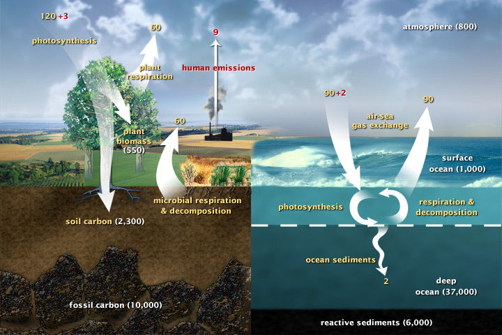
The carbon cycle describes the flow of carbon between resevoirs in the Earth system. The largest pools of carbon are fossil carbon, deep ocean and reactive sediments, soil carbon, carbon at the ocean surface, and that in the atmosphere. After these comes that stored in plant biomass. Processes of photosynthesis, respiration and decomposition, as well as gas interchange at the ocean surface move carbon between the different pools. On top of that, we have the impact of anthropogenic emissions, which as we have seen above is injecting around 9 (8.749 using the 2008 figures above) Gigatons of carbon a year into the atmosphere from fossil fuel combustion.
A small aside on units:
8.749 * 3.667 * 1000 = 32082.6 Tg CO2 equivalent which is the figure quoted above. See CDIAC information on reporting units for details). Using 5.137 x 10¹⁸ kg as the mass of the atmosphere (Trenberth, 1981 JGR 86:5238-46), 1 ppmv of CO2 = 2.13 Gt of carbon (CDIAC FAQ). So, 8.749 Gt of carbon is equivalent to 4.11 ppmv of CO2.
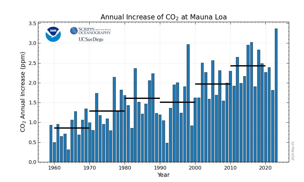
The annual mean growth rate of CO2 in the atmosphere is currently over 2 ppmv of CO2, from which it can be inferred that just over 2 ppmv of CO2 must enter other fast pools of carbon.
A view of the carbon cycle with more detail, from the IPCC AR5 is:
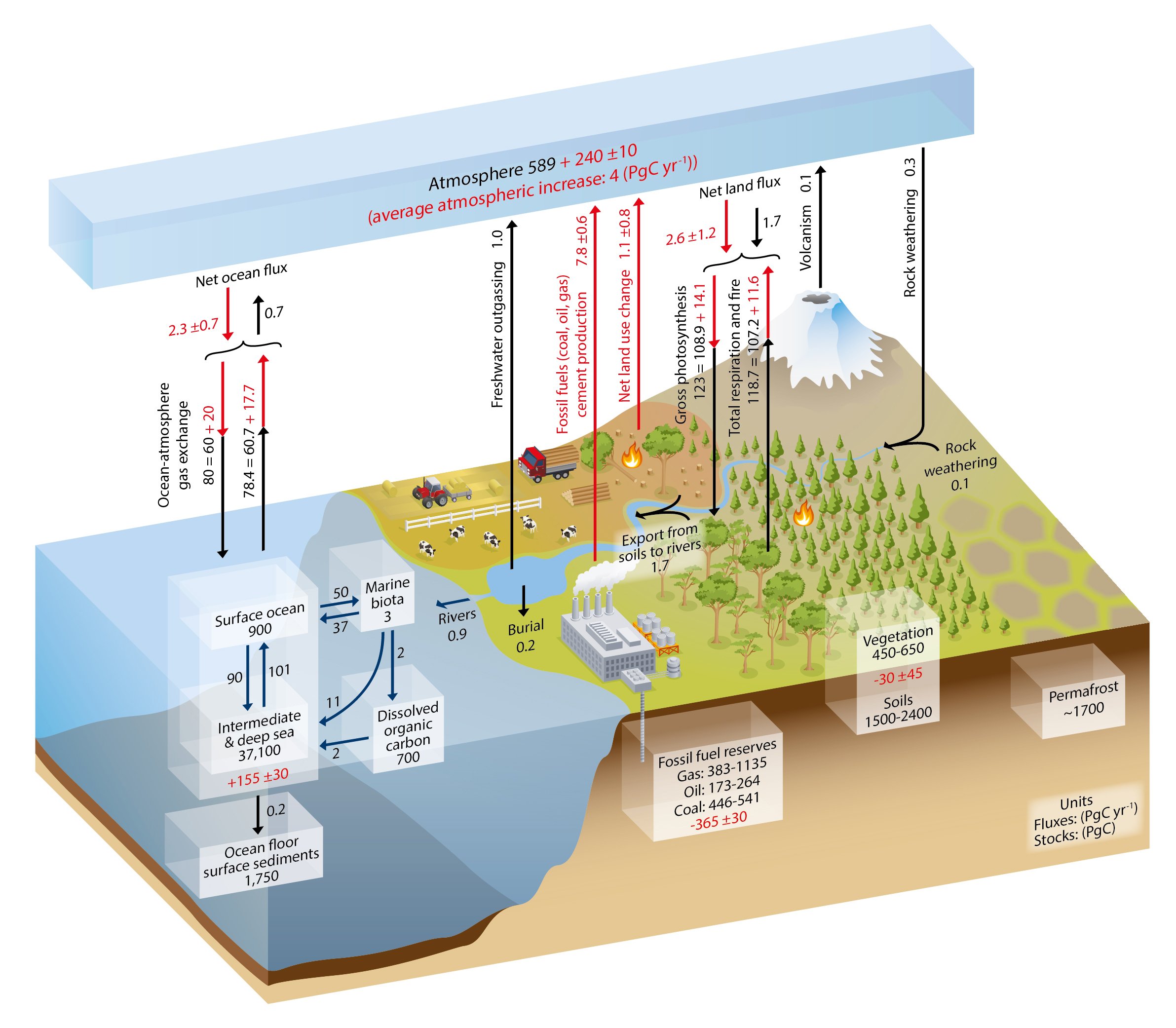

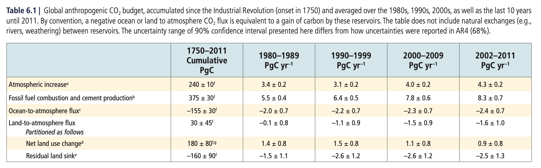
The increase in atmospheric CO2 is around 4.3 (+/- 0.2) PgCy^-1 (2002-2011 figures). The table above shows how this is partitioned from the main sources and sinks. Despite being the smallest flux, the Land-to-atmosphere flux has the largest uncertainty. Note that the ‘Residual land sink’ is calculated to balance the budget, rather than being a direct caclulation.
3.2.1. Uncertainties

The figure above illustrate what is currently known about both the magnitudes and uncertainties of what the global carbon cycle fluxes were in the 1990s. The increase in atmospheric carbon is less than that emitted from burning fossil fuels as discussed above. The balance is made up of net flows to the ocean and land. The largest uncertainty is in the net terrestrial uptake even though this is the smallest component of the flux. The land sink involves emissions from fire and land use change and a land carbon sink which has the greatest uncertainty of the sub components(0.9 to 4.3 Gt carbon yr-1). Estimates stocks of land carbon are also shown, which indicate a terrestrial vegetation pool of around 600 Gt of carbon (similar order of magnitude to that in the atmosphere) and a much larger but less mobile (on decadal to annual time scales) soil and detritus pool.


The figure below shows net and gross CO2 fluxes from the land, separating these into Agriculture, Forestry and Other Land Use (AFOLU) and indirect emissions and removals. The uncertainty on the gross indirect fluxes is particularly high. The total net land flux (removal) is currently estimated to be on average (2007-2016) around 6.0 +/- 2.0 GtCO2y^-1 (AR5). One ton of carbon equals 3.67 tons of carbon dioxide, so this equates to 1.63 +/- 0.54 GtCy-1.
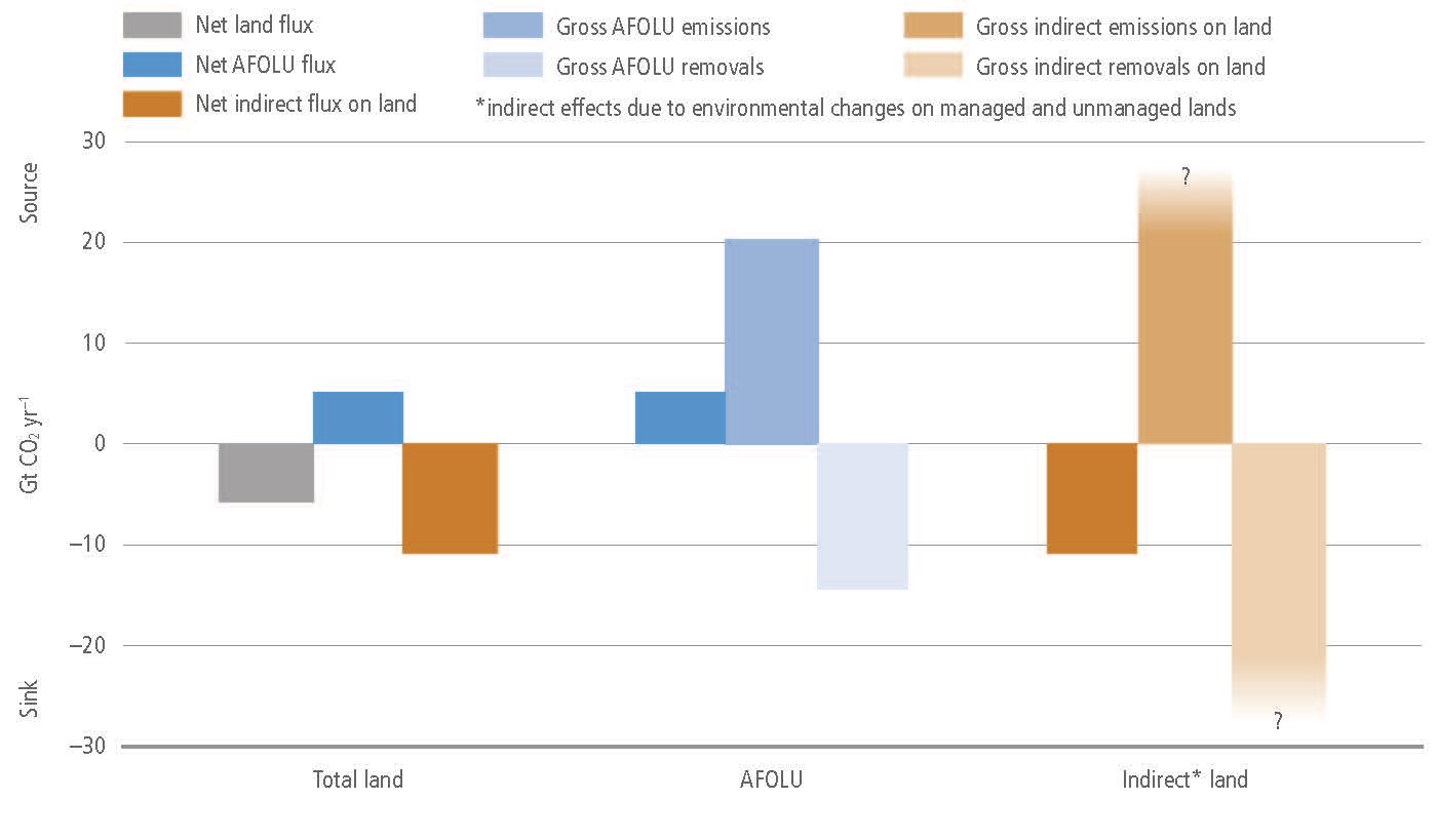
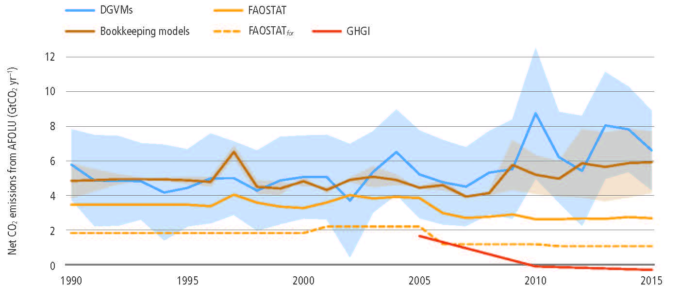
Trying to reconcile the net land sink is complicated then, partly because of the large and competing components and also through a lack of real constraint on indirect fluxes. Further, even though countries report their annual AFOLU (and other) fluxes to the UN (GHG inventory), these are currently quite different from other estimates of the fluxes, from modelling or from bookkeeping models:
3.3. Biogeochemical processes
3.3.1. Net Ecosystem CO2 flux
As we saw above, the global annual flux of carbon to the atmosphere from microbial respiration and decomposition is thought to be around 120 Gt of carbon per year. This is approximately balanced by the process of photosynthesis that currently draws down around 123 Gt of carbon per year, including around 3 Gt attributed to anthropogenic inputs into the atmosphere that goes into the land sink.
Arriving at figures like that is complex for many reasons, so we have to think carefully about what we measure and model and also precisely define the terms we use. Lovett et al., (2006) provides a useful discussion of carbon flows in an ecosystem and the terms you will need to be aware of.
We can consider CO2 fluxes at the ecosystem level:
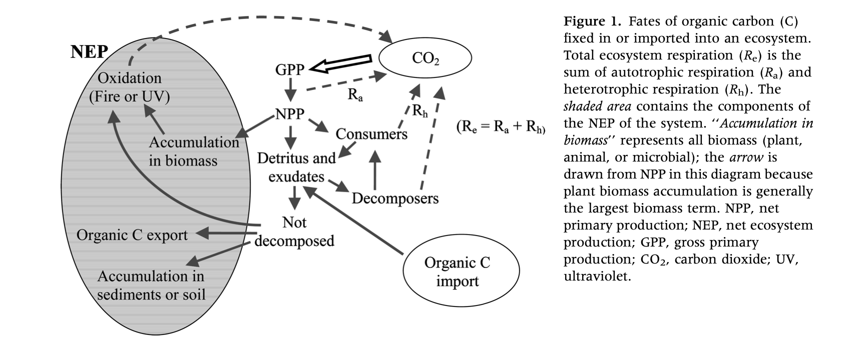
Gross Primary Productivity (GPP) is the amount of carbon (per unit area per unit time) taken up by green vegetation in the ecosystem, which is simply the photosynthetic rate (at the ecosystem level). Photosynthesis involves the use of (solar) energy to convert CO2 and H20 to glucose (C6H12O6) and oxygen (O2).
Plants use (metabolise) energy (burn carbohydrates) to maintain growth, reproduction and other life processes. This is the process of (autotrophic) respiration (\(R_a\)), which releases CO2 (and water) to the atmosphere. Additional respiration by soil micro-organisms and soil animals (consumers and decomposers) in the decomposition of soil organic matter is known as heterotrophic respiration (\(R_h\)). The total ecosystem respiration then, \(R_e\) is the sum of \(R_a\) and \(R_h\).
The net ecosystem productivity (NEP) is defined:
In this way, it represents the organic C available for storage within the ecosystem or that can be transported out of the ecosystem as a loss (e.g. fire or harvest). The sign of NEP indicates whether there is a net input to (positive NEP) or output from (negative NEP) the system. Lovett et al., (2006) note that this is not quite the same as the change in C storage, as that should include any imports and exports of organic C (e.g. fertilizer, wood harvesting) and non-biological oxidation of C.
The related term, Net Ecosystem Exchange (NEE), is essentially equal to NEP but opposite in sign (i.e. NEE is negative when GPP is higher than \(R_e\)). Technically, it also includes sources and sinks for CO2 that do not involve conversion to or from organic C (e.g. weathering reactions), but these will tend to be minor for terrestrial ecosystems, and NEE is mostly treated and -NEP.
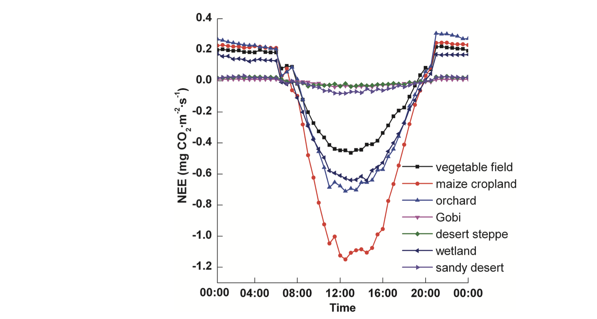
The figure above shows typical diurnal variations in CO2 fluxes over some vegetation canopies. The measure given is Net Ecosystem Exchange (net CO2 flux) (units: mg CO2 m-2 s-1). During the daytime, the fluxes are negative (i.e. there is a flow from the atmosphere to the ecosystem) and at nighttime, the flux (to the atmosphere) is positive (so the ecosystem loses CO2 to the atmosphere).
Ecosystem-level measures are of great value as they integrate all of the processes involved with plants, animals and soil, over some specified spatial and temporal domain. They are also things that we can measure, e.g. using eddy covariance towers, as we shall see later.
However, we also need to be able to model, measure and understand the processes underlying this which means considering the plant level. This is often not considered practically possible, so we group plants together that we want to consider as a set, or that we believe operate in a similar manner. Of course several, or many individual plants will form part of an ecosystem. This may sometimes then be considered as a ‘layer’ of vegetation (e.g. a tree canopy) or as several layers (canopy and understory). Such ‘layer’ separation can be important if the responses and timing of events in the different layers varies, as is often the case for a tree canopy and understory.
Taking all green plants in the ecosystem together then, we can try to isolate and define some of the ‘plant-scale’ processes. A critical term in this sense is net primary productivity (NPP), which is effectively the rate of biomass production. This is defined as ecosystem GPP minus plant respiration losses (\(R_a\)):
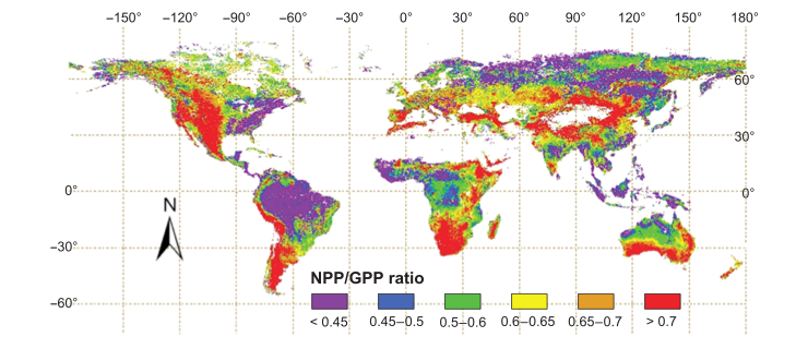
The ratio of NPP to GPP is known as the carbon use efficiency (CUE). This is the fraction of carbon absorbed by an ecosystem that is used in biomass production, and is quite similar across ecosystems, typically assumed to be around 0.5. DeLucia et al. (2007) for example confirm an average value of 0.53 across many forest ecosystems, but they note that individual values of CUE can range from 0.23 to 0.83.
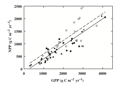
Similarly, Zhang et al. (2009) showed that CUE exhibited a pattern depending on the main climatic characteristics such as temperature and precipitation and geographical factors such as latitude and altitude.

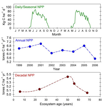
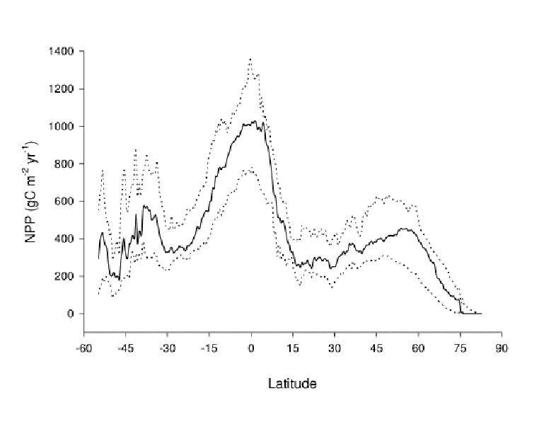
NPP varies over the year as the factors affecting the processes involed (essentially, light, temperature and water availability) vary over the growing seasdon. Nutrient availability also affects NPP but this is likely to vary over longer time periods. NPP can very quite significantly from one year to the next and over decadal timescales depending on climatic factors.
NPP varies quite considerably between biomes. The following table shows typical values of GPP, total Global NPP and NPP per unit area for the main biomes.
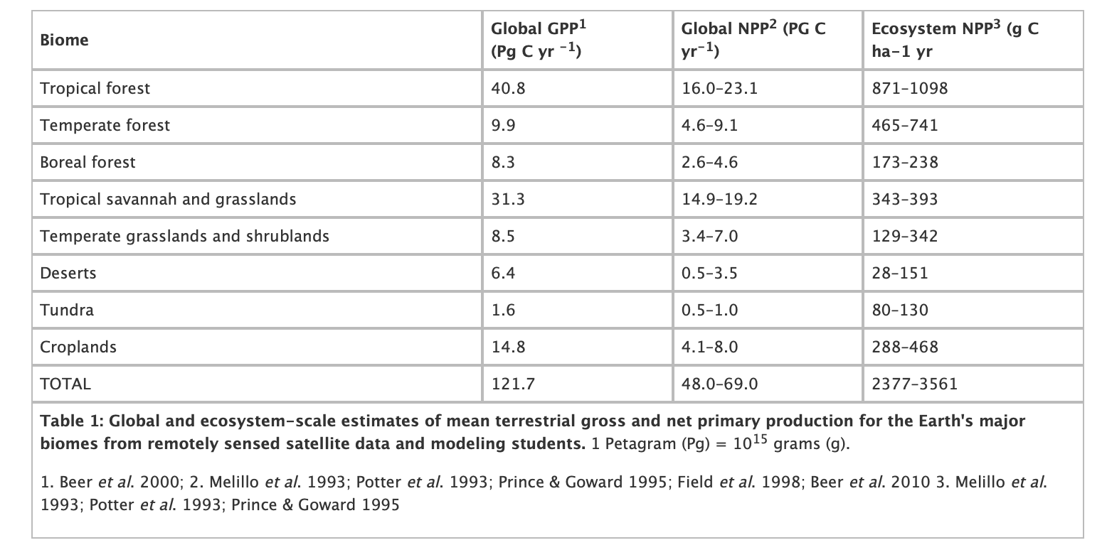
Globally then, the most productive biomes are tropical forests, savannah and grassland which together account for around half of global NPP, and the predominance of the tropics can be seen in the figure below. But per unit area, tropical and temperate forests are the most productive.

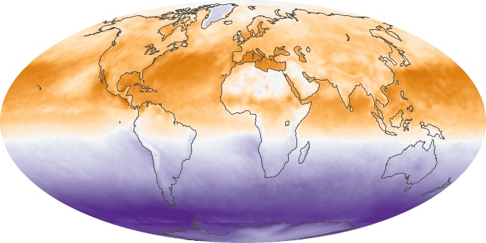
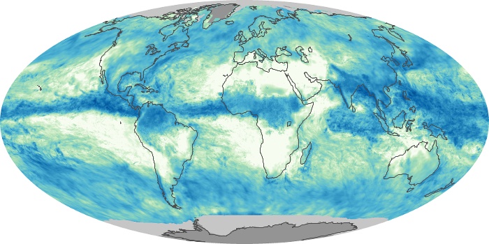
The figures above show global NPP distribution and related climatic and land surface properties for Northern hemisphere summer. The dataset ‘NPP’ broadly relates the abundance of vegetation, which relates to the total capacity of vegetation to photosynthesise. The primary driver of GPP (so NPP in broad terms) is the amount of vegetation and the amount of downwelling solar radiation. Although we do not have an image of the latter here, it is broadly in-line with the net radiation shown. There are of course many more subtle controls on NPP that we will consider later, but clearly these would include temperature range and water availability.
In Northern hemisphere summer then, NPP is most strongly spatially weighted to the Northern hemisphere because of these various drivers.

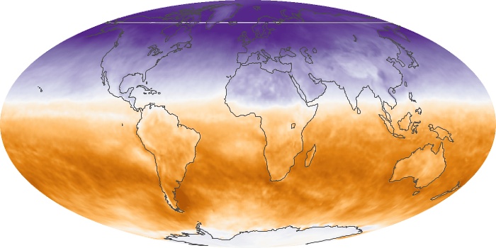
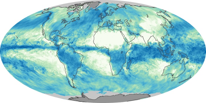
In Northern hemisphere winter, the distribution of NPP shifts to the Southern hemisphere, for the same reasons as indicated above.
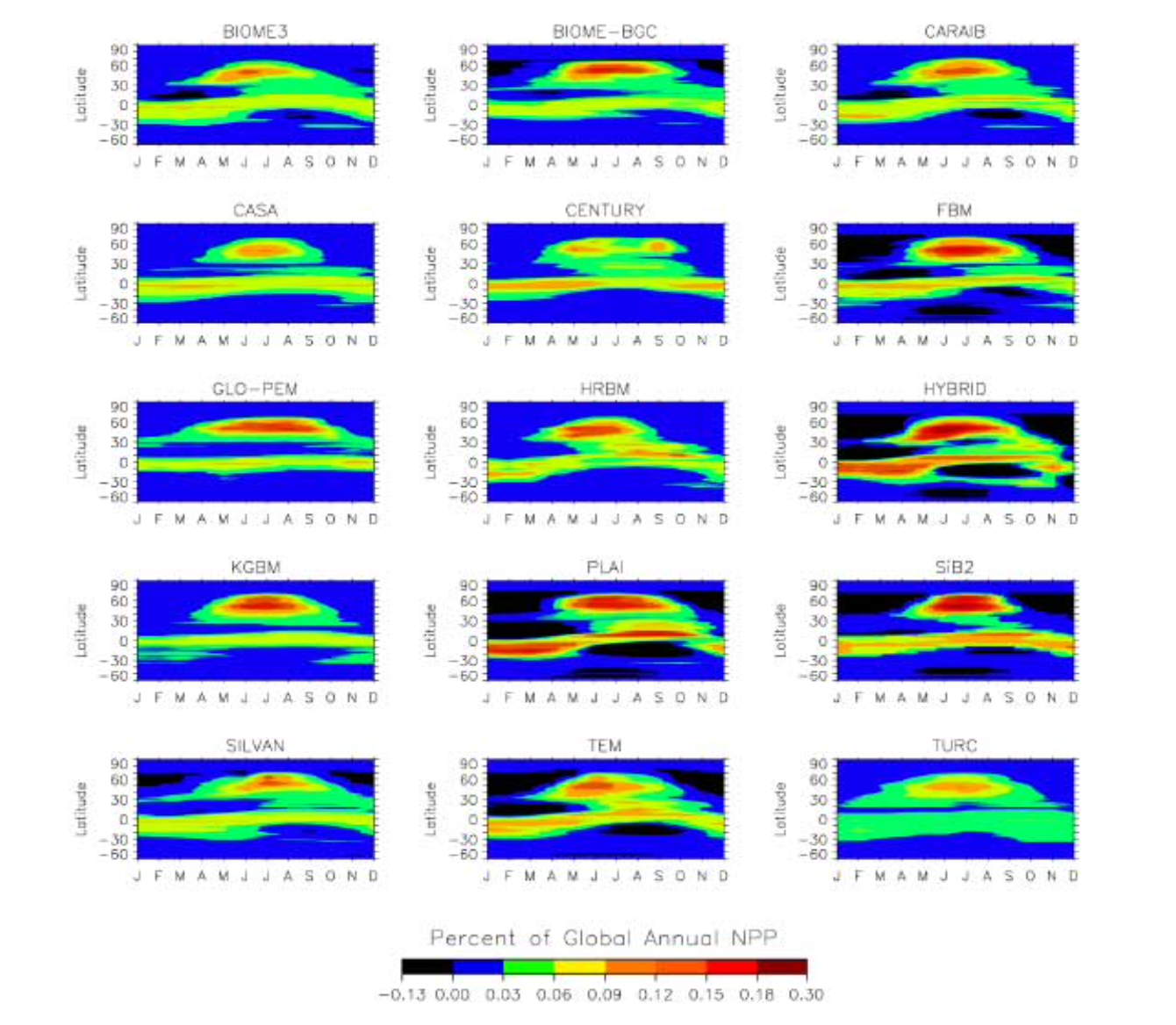
Since the total landmass (and in particular the vegetated landmass) in the Southern hemisphere is less than that of the Northern hemisphere, global NPP comes predominantly from Northern latitudes. Referring back to the plots of the annual cycle of atmospheric CO2 above, we noted a peak in May and a trough in October, largely then in response to global NPP increases in Spring and decreases in Autumn: the larger NPP in Northern hemisphere summer gradually decreases the atmospheric CO2 concentration. This is however complicated by the timing and spatial distribution of other CO2 sources and sinks.
3.3.2. Net Ecosystem Productivity
The NEP then is NPP minus other losses to the atmosphere. These will generally include respiration by heterotrophs (organisms – fungi, animals and bacteria in the soil), but there may be other losses to the ecosystem such as through harvesting or fire.
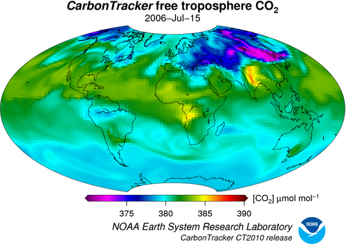
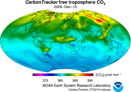
Anthropogenic and wildfire carbon emissions (as well as ocean and soil fluxes) as well as atmospheric circulation also significantly affect the global distribution of CO2, so the global patterns of CO2 are not as ‘simple’ as just the NPP fluxes.
3.4. Summary
In this lecture, we have:
looked in detail at the terrestrial carbon cycle
provided an overview of relevant biogeochemical processes
3.5. Reading for this lecture
Texts of particular importance to this lecture are:
Ryu et al., 2019, What is global photosynthesis? History, uncertainties and opportunities,Remote Sensing of Environment, https://doi.org/10.1016/j.rse.2019.01.016.
Heimann, M., Reichstein, M. Terrestrial ecosystem carbon dynamics and climate feedbacks. Nature 451, 289–292 (2008). https://doi.org/10.1038/nature06591
Forests and Climate Change: Forcings, Feedbacks, and the Climate Benefits of Forests, G.B. Bonan, Science 320, 1444 (2008), DOI: 10.1126/science.1155121
Monteith, J.L. and Unsworth, M., (2007), Principles of Environmental Physics, Academic Press
Forseth, I. (2010) Terrestrial Biomes. Nature Education Knowledge 1(8):12
Grace, J., (2001) Carbon Cycle, in Encyclopedia of Biodiversity, Vol. 1, Academic Press
DeLucia et al. (2007) Forest carbon use efficiency: is respiration a constant fraction of gross primary production? Global Change Biology (2007) 13, 1157–1167, doi: 10.1111/j.1365-2486.2007.01365.x
Lovett, G.M. et al., (2006) Is Net Ecosystem Production Equal to Ecosystem Carbon Accumulation? Ecosystems (2006) 9: 1–4 DOI: 10.1007/s10021-005-0036-3
Gough, C. M. (2011) Terrestrial Primary Production: Fuel for Life. Nature Education Knowledge 2(2):1